Use this file to discover all available pages before exploring further.
View on GitHub
Open this notebook in GitHub to run it yourself
This notebook relates to the paper “Optimization by Decoded Quantum Interferometry” (DQI) [1], which introduces a quantum algorithm for combinatorial optimization problems.The algorithm focuses on finding approximate solutions to the max-LINSAT problem, and takes advantage of the sparse Fourier spectrum of certain optimization functions.
Input: A matrix B∈Fm×n and m functions fi:F→{+1,−1} for i=1,⋯,m, where F is a finite field.
Define the objective function f:Fn→Z to be f(x)=∑i=1mfi(∑j=1nBijxj).
Output: a vector x∈Fn that best maximizes f.
The paper shows that for the problem of Optimal Polynomial Intersection (OPI)—a special case of the the max-LINSAT—the algorithm can reach a better approximation ratio than any known polynomial time classical algorithm.We demonstrate the algorithm in the setting of max-XORSAT, which is another special case of max-LINSAT, and is different from the OPI problem.Even though the paper does not show a quantum advantage with max-XORSAT, it is simpler to demonstrate.
Input: A matrix B∈F2m×n and a vector v∈F2m with m>n.
Define the objective function f:F2n→Z as f(x)=∑i=1m(−1)vi+bi⋅x=∑i=1mfi(x) (with bi the columns of B), which represents the number of satisfied constraints minus the number of unsatisfied constraints for the equation Bx=v.
Output: a vector x∈F2n that best maximizes f.
The max-XORSAT problem is NP-hard. As an example, the Max-Cut problem is a special case of max-XORSAT where the number of ones in each row is exactly two.The DQI algorithm focuses on finding approximate solutions to the problem.
The strategy is to prepare this state:∣P(f)⟩=x∈F2n∑P(f(x))∣x⟩where P is a normalized polynomial.Choosing a good polynomial can bias the sampling of the state towards high f values.The higher the degree l of the polynomial, the better approximation ratio of the optimum we can get.The Hadamard spectrum of ∣P(f)⟩ isk=0∑l(km)wky∈F2m∣y∣=k∑(−1)v⋅y∣BTy⟩where wk are normalized weights that can be calculated from the coefficients of P. So, to prepare ∣P(f)⟩, we prepare its Hadamard transform, then apply the Hadamard transform over it.Stages:
Prepare ∑k=0lwk∣k⟩.
Translate the binary encoded ∣k⟩ to a unary encoded state ∣k⟩unary=∣k1⋯1n−k0⋯0⟩, resulting in the state ∑k=0lwk∣k⟩unary.
Translate each ∣k⟩unary to a Dicke state [2], resulting in the state ∑{k=0}{l}w{k}{{(m{)}{k}}}∑{{y∈{F}2m∣y∣=k}}∣y⟩m.
For each ∣y⟩m, calculate (−1)v⋅y∣y⟩m∣BTy⟩n, getting ∑{k=0}{l}w{k}{{(m{)}{k}}}∑{{y∈{F}2m∣y∣=k}}(−1){v⋅y}∣y⟩m∣BTy⟩n.
Uncompute ∣y⟩m by decoding ∣BTy⟩n.
Apply the Hadamard transform to get the desired ∣P(f)⟩.
Step 5 is the heart of the algorithm.The decoding of ∣BTy⟩n is, in general, an ill-defined problem, but when the hamming weight of y is known to be limited by some integer l (the degree of P) , it might be feasible and even efficient, depending on the structure of the matrix B.The problem is equivalent to the decoding error from syndrome [3], where BT is the parity-check matrix.Figure 1 shows a layout of the resulting quantum program.Executing the quantum program guarantees that we sample x with high f values with high probability (see the last plot in this notebook).*Figure
The full DQI circuit for a MaxCut problem.
The x solutions are sampled from the target variable after the last Hadamard transform.*
Binary encoding: Represents a number using binary bits, where each qubit corresponds to a binary place value.
For example, the number 3 on 4 qubits is ∣1100⟩.
One-hot encoding: Represents a number by activating a single qubit, with its position indicating the value.
For example, the number 3 on 4 qubits is ∣0001⟩.
Unary encoding: Represents a number by setting the first k qubits to 1 k is the number, and the rest to
For example, the number 3 on 4 qubits is ∣1110⟩.
Specifically, we translate a binary (unsigned QNum) to one-hot encoding, and show how to convert the one-hot encoding to a unary encoding.The conversions are done in place, meaning that the same binary encoded quantum variable is extended to represent the target encoding.We use the library function binary_to_unary, based on this post. Let’s test the conversion of the number 8 from binary to unary:
We transform a unary input quantum variable to a Dicke state, such thatU∣k1⋯1n−k0⋯0⟩=k=0∑l(kn)1∣y∣=k∑∣y⟩nWe use the library function prepare_dicke_state, with a recursive implementation that is based on [2].The recursion works bit by bit.We test the function for the Dicke state of 6 qubits with 4 ones:
In the DQI setting, we will want to prepare a Dicke state given a unary encoded quantum variable. We will use the function prepare_dicke_state_unary_input, which is actually a subrutine of prepare_dicke_state:
Define a matrix and vector product over the binary field functions:
from functools import reducefrom classiq.qmod.symbolic import pi@qfuncdef vector_product_phase(v: CArray[CInt], y: QArray): phase(pi * sum(v[i] * y[i] for i in range(v.len)))@qfuncdef matrix_vector_product(B: list[list[int]], y: QArray, out: Output[QArray]): allocate(len(B), out) for i in range(len(B)): out[i] ^= reduce( lambda x, y: x ^ y, [int(B[i][j]) * y[j] for j in range(y.len)] )
Here, we combine all the building blocks into the full algorithm. To save qubits, the decoding is done in place, directly onto the ∣y⟩ register.The only remaining part is the decoding, that will be treated after choosing the problem to optimize, as it depends on the input structure.dqi_max_xor_sat is the main quantum function of the algorithm. It expects the following arguments:
B: the (classical) constraints matrix of the optimization problem
v: the (classical) constraints vector of the optimization problem
w_k: a (classical) vector of coefficients wk corresponding to the polynomial transformation of the target function.
The index of the last non-zero element sets the maximum number of errors that the decoder should decode
y: the (quantum) array of the errors for the decoder to decode. If the decoder is perfect, it should hold only zeros at the output
solution: the (quantum) output array of the solution. It holds ∣BTy⟩ before the Hadamard transform.
syndrome_decode: a quantum callable that accepts a syndrome quantum array and outputs the decoded error on its second quantum argument
@qfuncdef dqi_max_xor_sat( B: list[list[int]], v: list[int], w_k: list[float], y: Output[QArray], solution: Output[QArray], syndrom_decode: QCallable[QArray, QArray],): k_num_errors = QNum() prepare_amplitudes(w_k, 0, k_num_errors) k_unary = QArray() binary_to_unary(k_num_errors, k_unary) # pad with 0's to the size of m pad_zeros(B.len, k_unary, y) # Create the Dicke states max_errors = int(np.nonzero(w_k)[0][-1]) if np.any(w_k) else 0 prepare_dicke_state_unary_input(max_errors, y) # Apply the phase vector_product_phase(v, y) # Compute |B^T*y> to a new register matrix_vector_product(np.array(B).T.tolist(), y, solution) # uncompute |y> # decode the syndrom inplace directly on y syndrom_decode(solution, y) # transform from Hadamard space to function space hadamard_transform(solution)
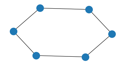
Now, let’s be more specific and optimize a Max-Cut problem. We choose specific parameters so that with the resulting B matrix we can decode up to two errors on the vector ∣y⟩.The translation between Max-Cut and max-XORSAT is quite straightforward.Every edge is a row, with the nodes as columns.The v vector is all ones, so that if (vi,vj)∈E, we get a constraint xi⊕xj=1, which is satisfied if xi, xj are on different sides of the cut.
import itertoolsimport warningsimport matplotlib.pyplot as pltimport networkx as nxwarnings.filterwarnings("ignore", category=FutureWarning)# A 2-regular graph on 6 nodesG = nx.Graph()G.add_nodes_from([3, 4, 1, 5, 2, 0])G.add_edges_from([(3, 4), (3, 2), (4, 1), (1, 5), (5, 0), (2, 0)])B = nx.incidence_matrix(G).T.toarray()v = np.ones(B.shape[0])plt.figure(figsize=(4, 2))nx.draw(G)print("B matrix:\n", B)
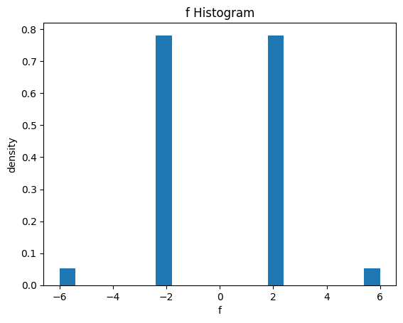
Let’s plot the statistics of f for uniformly sampling x, as a histogram.Later, we show how to get a better histogram after sampling from the state of the DQI algorithm.
# plot f statisticsall_inputs = np.array(list(itertools.product([0, 1], repeat=B.shape[1]))).Tf = ((-1) ** (B @ all_inputs + v[:, np.newaxis])).sum(axis=0)# plot a histogram of fplt.hist(f, bins=20, density=True)plt.xlabel("f")plt.ylabel("density")plt.title("f Histogram")plt.show()
The transposed matrix of the specific matrix we have chosen can be decoded with up to two errors, which corresponds to a polynomial transformation of f of degree 2 in the amplitude, and degree 4 in the sampling probability:
# set the code length and possible number of errorsMAX_ERRORS = 2 # l in the papern = B.shape[0]# Generate all vectors in one lineerrors = np.array( [ np.array([1 if i in ones_positions else 0 for i in range(n)]) for num_ones in range(MAX_ERRORS + 1) for ones_positions in itertools.combinations(range(n), num_ones) ])syndromes = (B.T @ errors.T % 2).Tprint("num errors:", errors.shape[0])print("num syndromes:", len(set(tuple(x) for x in list((syndromes)))))print("B shape:", B.shape)
For this basic demonstration, we use a brute force decoder that uses a lookup table for decoding each syndrome in superposition:
def _to_int(binary_array): return int("".join(str(int(bit)) for bit in reversed(binary_array)), 2)@qfuncdef syndrome_decode_lookuptable(syndrome: QNum, error: QNum): for i in range(len(syndromes)): control( syndrome == _to_int(syndromes[i]), lambda: inplace_xor(_to_int(errors[i]), error), )
It is also possible to define a decoder that uses a local rule of syndrome majority.This decoder can correct just one error.
@qfuncdef syndrome_decode_majority(syndrome: QArray, error: QArray): for i in range(B.shape[0]): # if 2 syndromes are 1, then the decoded bit will be 1, else 0 synd_1 = np.nonzero(B[i])[0][0] synd_2 = np.nonzero(B[i])[0][1] error[i] ^= syndrome[synd_1] & syndrome[synd_2]
According to the paper [1], this is done by finding the principal value of a tridiagonal matrix A defined by the following code.The optimality is with regard to the expected ratio of satisfied constraints.
def get_optimal_w(m, n, l): # max-xor sat: p = 2 r = 1 d = (p - 2 * r) / np.sqrt(r * (p - r)) # Build A matrix diag = np.arange(l + 1) * d off_diag = [np.sqrt(i * (m - i + 1)) for i in range(1, l + 1)] A = np.diag(diag) + np.diag(off_diag, 1) + np.diag(off_diag, -1) # get W_k as the principal vector of A eigenvalues, eigenvectors = np.linalg.eig(A) principal_vector = eigenvectors[:, np.argmax(eigenvalues)] # normalize return principal_vector / np.linalg.norm(principal_vector)# normalizeW_k = get_optimal_w(m=B.shape[0], n=B.shape[1], l=MAX_ERRORS)print("Optimal w_k vector:", W_k)# complete W_k to a power of 2 for the usage in prepare_stateW_k = np.pad(W_k, (0, 2 ** int(np.ceil(np.log2(len(W_k)))) - len(W_k)))
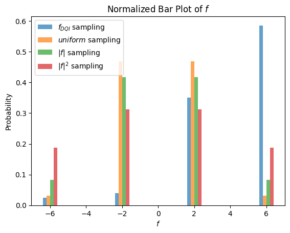
Finally, we plot the histogram of the sampled f values from the algorithm, and compare it to a uniform sampling of x values, and also to sampling weighted by ∣f∣ and ∣f∣2 values. We can see that the DQI histogram is biased to higher f values compared to the other sampling methods.
import matplotlib.pyplot as pltimport numpy as np# Example data initializationf_sampled = []shots = []# Populate f_sampled and shots based on res.parsed_countsfor sample in res.parsed_counts: solution = sample.state["solution"] f_sampled.append(((-1) ** (B @ solution + v)).sum()) shots.append(sample.shots)f_sampled = np.array(f_sampled)shots = np.array(shots)unique_f_sampled, indices = np.unique(f_sampled, return_inverse=True)prob_f_sampled = np.array( [shots[indices == i].sum() for i in range(len(unique_f_sampled))])prob_f_sampled = prob_f_sampled / prob_f_sampled.sum()f_values, f_counts = np.unique(f, return_counts=True)prob_f_uniform = np.array(f_counts) * np.array(f_values)prob_f_uniform = f_counts / sum(f_counts)prob_f_abs = np.array(f_counts) * np.array(np.abs(f_values))prob_f_abs = prob_f_abs / prob_f_abs.sum()prob_f_squared = np.array(f_counts) * np.array(f_values**2)prob_f_squared = prob_f_squared / prob_f_squared.sum()# Plot normalized bar plotsbar_width = 0.2plt.bar( unique_f_sampled - 1.5 * bar_width, prob_f_sampled, width=bar_width, alpha=0.7, label="$f_{DQI}$ sampling",)plt.bar( f_values - 0.5 * bar_width, prob_f_uniform, width=bar_width, alpha=0.7, label="$uniform$ sampling",)plt.bar( f_values + 0.5 * bar_width, prob_f_abs, width=bar_width, alpha=0.7, label="$|f|$ sampling",)plt.bar( f_values + 1.5 * bar_width, prob_f_squared, width=bar_width, alpha=0.7, label="$|f|^2$ sampling",)plt.title("Normalized Bar Plot of $f$")plt.xlabel("$f$")plt.ylabel("Probability")plt.legend()plt.show()print("<f_uniform>:", np.average(f))print("<f_DQI>:", np.average(f_sampled, weights=shots))