Use this file to discover all available pages before exploring further.
View on GitHub
Open this notebook in GitHub to run it yourself
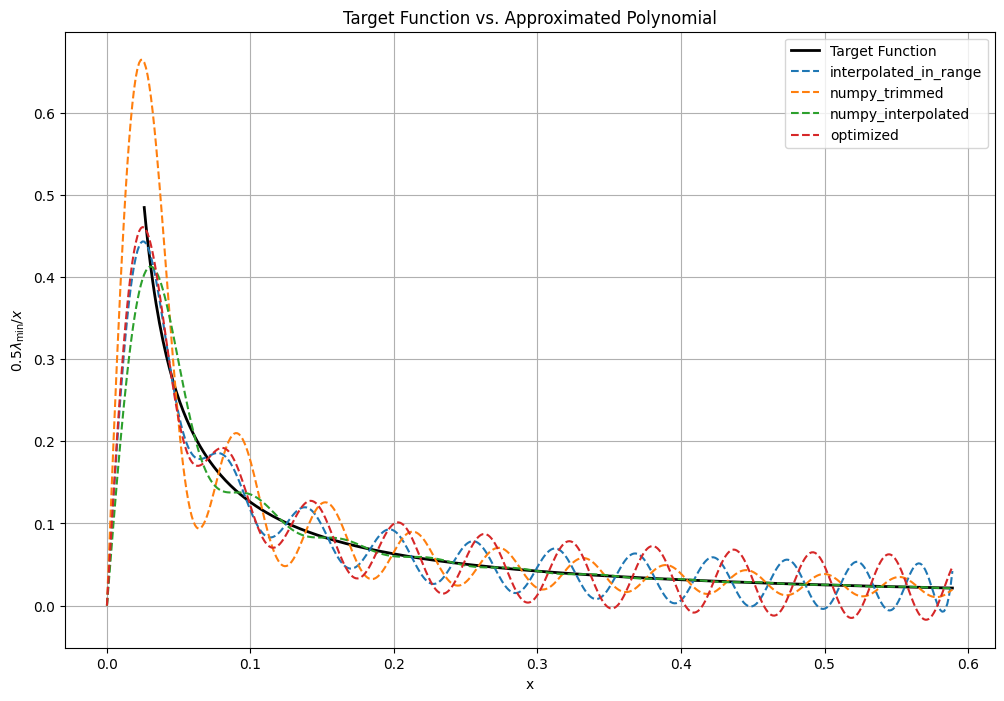
In this notebook we present the four ways of approximating the inverse function with Chebyshev polynomials:
Using Classiq’s QSP application.
Here the approximation can be made within an interval [\lambda_\min, \lambda_\max], and the polynomial values are bounded in [−1,1].
Using Numpy interpolation with a give degree, here the polynomial values are bounded in [−1,1].
Using Numpy interpolation with the theoretical degree, and then trimming to a smaller degree.
Using an optimized (for the Maximum norm) expansion according to https://arxiv.org/pdf/2507.15537 (available in Classiq QSP application).
import matplotlib.pyplot as pltimport numpy as npfrom cheb_utils import *from pauli_be import *from scipy import sparsefrom classiq.applications.chemistry.op_utils import qubit_op_to_qmod
import pathlibpath = ( pathlib.Path(__file__).parent.resolve() if "__file__" in locals() else pathlib.Path("."))
We upload some matrix, and considered its block-encoding. We need the block-encoding scaling factor in order to calculate the effective range of singular/eigen-values.
min singular value: 0.02516479472045721, max_singular value: 0.589120855859263
  For error 0.01, and given kappa, the needed polynomial degree is: 899
  Performing convex optimization for the Chebyshev interpolation, with degree 101
  For error 0.01, and given kappa, the needed polynomial degree is: 899
  Performing numpy Chebyshev interpolation, with degree 899 and trimming to degree 101
  For error 0.01, and given kappa, the needed polynomial degree is: 899
  Performing numpy Chebyshev interpolation, with degree 101
  For error 0.01, and given kappa, the needed polynomial degree is: 899
  Taking optimized expansion from literature, with degree 101