View on GitHub
Open this notebook in GitHub to run it yourself
Overview
This notebook implements a quantum simulation of the one-dimensional Fermi-Hubbard model using Classiq’s quantum programming framework. The simulation proceeds in three stages:- Initial state preparation — The ground state of a non-interacting Hamiltonian with a spin-dependent attractive potential is prepared as a Slater determinant via Givens rotations.
- Time evolution — The system is quenched to the interacting Fermi-Hubbard Hamiltonian and propagated using a first-order Trotterized circuit, where each Trotter step is decomposed into hopping and interaction layers using the Jordan-Wigner transformation.
- Measurement and analysis — Charge and spin densities are measured at each time step to observe the dynamics, testing the phenomenon of spin-charge separation at intermediate interaction strengths.
Introduction
The Fermi-Hubbard model is a fundamental corner step of condensed matter physics, describing the interplay between kinetic energy and repulsion interaction between electrons in a solid. Although very simple, in certain parameter regimes, the model showcases a variety strongly correlated phenomena, such as the metal-insulator transition (Mott physics), antiferromagnetism, inhomogeneous phases, and unconventional Fermi liquids. In order to motivate or conceptually derive the model, consider of a metalic material composed of atoms organized in a regular pattern, i.e., a lattice. We assume the temperature is sufficiently low, so the that the vibrations of the atoms can be neglected and the atoms are essentially held in a fix position in the lattice sites. Moreover, typically each atom has a handful of relevant energy levels, however, in order to simplify the problem we will consider only a single energy level at each lattice site (one energy level per atom). In the metal, valance electrons move freely between the metal atoms, leading to the expected conductive behaviour. The movement of the electrons between the sites is dictated by the overlap of the spatial wave function on different sites. Since the atomic wave-functions decay exponentially with the distance to the nuclei, we consider only the dominant contribution, giving rise to hopping of electrons only between adjacent lattice sites. These consideration lead to the first the hopping term, constituting the kinetic energy contribution: , where is the fermionic annihilation operator on the ‘th lattice site and spin. In addition, designates that the sum is only over nearest-neighbors. A second contribution arises from the repulsive Coulomb interaction between two electrons. Such interaction is strongest between electrons on the same atom. We consider only this dominant contribution, adding an energy penalty of , for two-electrons on the same site. In addition, Pauli’s exclusion principle dictates that two electrons cannot be in the same quantum state, therefore the repulsive interaction can only be between electrons with different spins: . Overall, the Fermi-Hubbard Hamiltonian is given by: where is the number operator. The model constitutes a key tool in the investigation of transition metal oxides, organic conductors and cuprates, which exhibit high-temperature superconductivity and exotic quantum magnetism properties and unconventional symmetry breaking. Despite its apparent simplicity, the model is notoriously challenging, in 1D the Fermi-Hubbard model is solvable via Bethe ansatz [2], while the 2D and 3D cases have not exact solution (for general hopping and interaction coefficients, and ). However, in 3D quantum phenomena are suppressed and the model typically exhibit classical behaviour, well described by mean-field theories. Numerical studies are also limited beyond specific doping regimes (doping modifies the fraction of electrons/lattice sites). Perturbation theory becomes invalid when strong correlations between the electron emerge, while Monte-Carlo methods are restricted by the sign problem away from half filling (at half filling the number of electrons equals the number lattice sites). The physics of the model are conveniently analysed by measuring the evolution of the spin densities We consider a simplified model consisting of a lattice of sites, and study the dynamics for an intermediate interaction strength, .Classiq Implementation
We implement the Hamiltonian simulation in three steps, utilizing Classiq’s built-in functions.- Initial state-preparation: Efficiently prepare the ground state of a non-interacting FH system in the presence of an external spin dependent potential.
- Time-evolution: Abruptly turn on the two-electron repulsion interaction and turn off the external potential, leading to dynamics governed by Hamiltonian (1).
- Measurement: The spin densities are evaluated.
Output:
Initial State Preperation
We begin by desribing a general algorithm to prepare Slater determinant states. Following, the algorithm is benchmarked on a simple example involving a four-by-four single particle hamiltonian. The state preperation algorithm is then utilized to prepare the ground state of the non-interacting Fermi-Hubbard Hamiltonian for the case of a single electron. This is then benchmarked against an analitical solution. Finally, we prepare on the initial state of the dynamic simulation, a ground state of the Fermi-Hubbard model for a quater-filling.Preparation of a Slater Determinant State
A Slater-Determinant is the ground state of a quadratic Fermionic Hamiltonian which conserves the number of particles. We begin by discussing an efficient algorithm to construct the initial non-interacting state. As all ground states of non-interacting fermionic Hamiltonian, the ground state is a fermionic Gaussian state, which can be prepared in a worst-case circuit depth of [3]. Specifically, for a quadratic Hamiltonian which conserves the number of particles, the fermionic Gaussian state can be expressed as a Slater determinant. For a general number conserving quadratic fermionic Hamiltonian where is known as the one-body Hamiltonian. Using the anti-commutation relations and the Heisenberg equation (), we have where the the time-dependence is suppressed for concisness. The dynamics in the Heisenberg representation can therefore be expressed as where and is the total number of fermionic modes. Remarkably, this implies that the diagonalization of , (an by matrix) provides the dynamics in the Hilbert space. Diagonalizing the single particle Hamiltonian , where is and -by- unitary matrix and , we obtain , where Alternatively, the basis transformation can be expressed in terms of the single-particle transformation, where we collected the creation operators to form an operator valued vector: and similarly for . For a fixed particle number the ground state is given by where iterates over the occupied fermionic modes and . The diagonalization of scales only polynomially with the number of lattice sites, and can be efficiently done on a classical computer. In order to prepare the desired ground state we focus on a part of which corresponds to the occupied modes, and denote the by matrix describing these modes by . This identification leads to an alternative form for Eq. (3), for the occupied modes we have An efficient quantum circuit for the ground state preparation can be obtained by a modified QR decomposition of , using a product of elementary two-mode rotations, called Given rotations. Each rotation can be expressed as \begin{pmatrix} \mathcal{G}c_k^\dagger\mathcal{G}\\ \mathcal{G}c_j^\dagger\mathcal{G} \end{pmatrix} = G(\theta,\varphi)\, \begin{pmatrix} c_k\\ c_j \end{pmatrix}~~, $ and the form of a Given rotation is $$G_\{jk\}(\theta,\varphi) = \begin\{pmatrix\} \cos(\theta) & -e^\{i\varphi\}\sin(\theta)\\ \sin(\theta) & e^\{i\varphi\}\cos(\theta) \end\{pmatrix\}~~. To simplify the decomposition we begin by utilizing the invariance of the Slater determinant (up to a global phase) under the mapping , where is a unitary transformation. For the transformation of basis to be valid we require that the first rows of are equal to , or alternatively Each Given transformation operates only on two columns and it’s parameters, and are set so to nullify elements in the upper right part of the matrix. Due to the orthogonality of the rows of , some transformations nullify more than a single matrix element. As a result, the total number of required Given transformations are , where is the number of electrons and is the number of fermionic modes. The diagonalization procedure results in a product of Given rotations After the Jordan-Wigner transformation, each two-mode () rotations correspond to a rotation in the single particle subspace of the two qubits and ( and ). This completely, defines the state preparation circuit in terms of a sequence two-qubit rotations. The gate complexity is (worst case achieved for ), and parallelization leads to a circuit depth of .Given Rotations Example
In order to understand the state preparation algorithm, we first show how Given rotations are utilized to diagonalize a simple one-body Hamiltonian. Consider a simple -by- Hermitian matrix, representing a one-body Hamiltonian: h = \begin\{pmatrix\} \varepsilon_0 & t_\{01\} & 0 & t_\{03\} \\ t_\{01\} & \varepsilon_1 & t_\{12\} & 0 \\ 0 & t_\{12\} & \varepsilon_2 & t_\{23\} \\ t_\{03\} & 0 & t_\{23\} & \varepsilon_3 \end\{pmatrix\} $QuadraticHamiltonian class in order to extract the Given rotations.
The number conserving quadratic Hamiltonian is then diagonalized utilizing a Bogoliubov transformation, leading to the orbital_energies and a transformation_matrix.
given_decomposition, returning a list of tuples: [(G_1,G_2),(G_3,),...]. Each tuple includes the Given rotations which can be operated in parallel. The Given rotations are encoded as a tuple: , where and are the columns of which the Given rotation is operated on from the right (see calculation below).
givens_gate implements the two-by-two matrix and build_U_from_rotations, gathers all the Given rotations to create .
Initial State Preparation of the Fermi Hubbard Model
The initial state is chosen to be the ground state of the non-interacting (i.e, quadratic in the fermionic creation/annihilation operators) Hamiltonian where the spin-up fermions feel a Gaussian attractive potential where spin-down fermions feel no potential, . The parameters , and dictate the precise shape and strength of the potential. Such potential creates a localized density peak of spin-up fermions and a flatter distribution for the spin-down fermions. As a result, the simulation begins with localized charge and spin densities. This state is generally not an eigenstate of the interacting Hamiltonian, constituting a highly excited (non-equilibrium) of the interacting system. We begin by defining a function mapping lattice and spin degrees of freedom to qubit number, these will assist us to associate fermionic degrees of freedom to the corresponding qubits in the quantum variables.givens_decomposition returns rotation parameters assuming the standard (little-endian) convention where the first qubit in the register is the least significant bit:
mode occupied, mode occupied.
Classiq’s unitary gate, however, uses big-endian ordering where the first qubit in the list is the most significant bit:
mode occupied, mode occupied.
Under the big-endian convention, the matrix as written above effectively implements (the inverse rotation) in the single-particle picture, introducing alternating sign errors in the prepared state amplitudes. To compensate, we swap the qubit order in the call to G, passing [qba[j], qba[i]] instead of [qba[i], qba[j]]. This restores the correct mode-to-index mapping so that the circuit faithfully implements the Givens rotations from the decomposition.
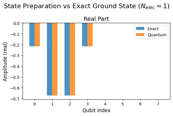
Single State Excitation Subspace Verification
For the single excitation subspace we can easily compare the preparation of the quantum state with the exact diagonalization. To compare between the two we normalize the quantum solution so to cancel the difference in the global phase with respect to the classical result.Output:
Output:
Initial State at Quater-Filling
At quater-filling the number of electrons equals to half number of lattice sites (quater of the fermionic modes). The one-body potential strength is set such that the two electrons will have different spins ()charge_density and spin_density which allow measuring the corresponding observables.
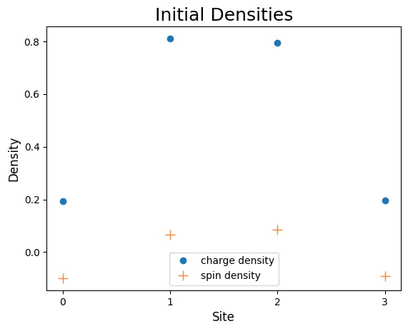
mean = , therefore the initial charge and spin densities form a peak around that site.
Time-Evolution
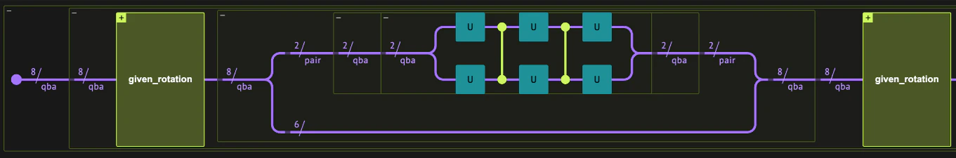
The propagation stage approximates the time-evolution operator , where is the 1D version of Eq. (1). The propagation of the initial state with respect to Eq. (4), simulates an effective quench of the system at initial time, abruptly changing the Hamiltonian . As a consequence, the initial state is a highly excited state of . In order to minimize the circuit depth of the quantum circuit it is beneficial to decompose the Hamiltonian into four sets of terms, where all the operators in a set commute with one another. The terms correspond to an even and odd edge hopping terms and even and odd site interaction terms: The odd hopping Hamiltonian term includes the hopping terms between and neighbouring sites ( is odd in Eq. (3)), while the odd hopping term includes the odd edge pairs (, , even ). The evolution operator is approximated by a first-order Trotter expansion, where each Trotter step consists of five stages. with Each component in the Trotter step can be achieved by simultaneous application (circuit depth of one) of simple two-qubit gates. An additional algorithmic trick simplifying the circuit and reducing the circuit depth even further. Between the even and odd interaction terms a fermionic mode swap operation is conducted, effectively performing a cyclic shifting of the fermionic modes. Crucially, this operation swaps the logical ordering of the qubits, while preserving the fermionic parity sign (using an iSWAP gates). Alternatively, the operation modifies the mapping between physical qubits and logical fermionic. As a result, the Hamiltonian terms are interpreted relative to the new ordering, effectively swapping the odd and even edge. The incorporation of the swap mode operation, allows parallelism, locality (only nearest neighbor gates, bypassing the need for long Jordan Wigner strings). After the application of an inverse fermionic mode swap is needed to swap the even and odd edges back, allowing application of the consecutive Trotter step. Since the even edge hopping term commutes with the inverse fermionic mod swap, these operations are merged to a single stage. Overall, the time-evolution involves iteration (each iteration corresponds to a single Trotter step) of a five-step procedure:- Hopping operation on odd edges.
- Interaction on odd sites
- Fermionic mode swap
- Interaction on even sites
- Hopping operation on even sites + inverse fermionic mode swap
K and P above implement the corresponding unitary transformations.
The first stage, including odd hopping terms, is obtained by simultaneous application of on different paris of qubits. Similarly, the second and fourth stages, involving the odd and even interactions are achieved with simultaneous application of on the corresponding pairs of qubits. The third stage, constituting the fermionic mode swap, is implemented by simultaneous iSWAP gates which is equivalent to . The last stage includes a merge of even-edge hopping operation, and an inverse fermionic mode swap operation. Naturally, since these operation commute, the transformation is obtained by two-qubit gates.
We implement the simultaneous operations on the qubit array utilizing Classiq’s built-in repeat function within the hop and interact functions.
Propagation and Execution (“Measurement”)
Output:
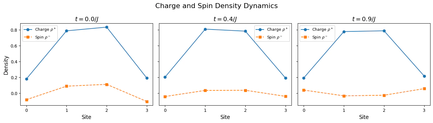
Analysis - Spin-Charge Separation
In order to quantify the spin-charge seperation, we evaluate the spin and charge spread: where . Different values between the spin and charge spreads, signifies spin-charge seperation.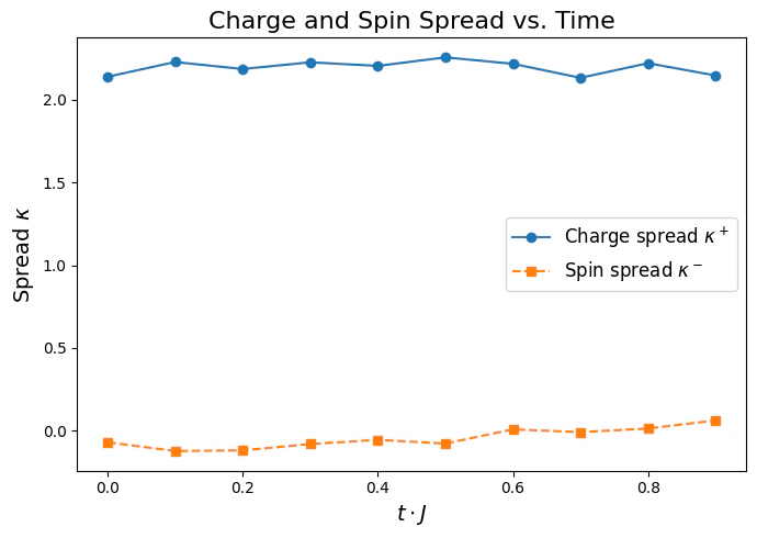
Comparison with Analytical Results
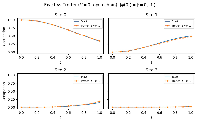
In order to validate the results, we compare the model prediction with the analytical solutions. There are two natural physical limits, where the model can be solved exactly and efficiently utilizing classical methods:- The non-interacting limit the on-site interaction vanishes (alternatively ).
- Vanishing hopping limit, (alternatively ).
Non-interacting Particles
In the non-interacting limit of , the FH Hamiltonian is a quadratic Hamiltonian. As a consequence, even in the case of site-dependent hopping or hopping between non-adjacent sites, the state dynamics can be solved classically in polynomial time in the number of fermionic modes , utilizing standard matrix exponentiation methods. In the case of the FH model on an open chain of sites, the non-interacting Hamiltonian becomes where n.i denotes “non-interacting”. The commutativity of the spin-up and spin-down terms allows them to be treated independently. For an open chain (no periodic boundary), the eigenstates are standing waves rather than plane waves. The single-particle eigenstates are with corresponding energies Each eigenstate is doubly degenerate (spin-up and spin-down). The ground state of an -electron system is obtained by filling the lowest-energy single-particle states one by one. The time-dependent expectation values of the charge and spin densities, , can readily obtained by employing the Heisenberg representation of quantum mechanics. In this representation, an operator’s, , dynamics is generated by the Heisenberg equation where , where . Substituting the diagonal form of and utilizing the fermionic anti-commutation relations (the Fourier fermionic operators satisfy similar commutation relations) we obtain , therefore , leading to The dynamics can be evaluated by introducing the matrices and with elements , this allows writting the dynamics of a second order correlation as In the one-excitation subspace, the ground state reads , where are the elements of the eigenstate of , i.e. , where is the ground state energy.Numerical Evaluation on a small model.
Defining parameters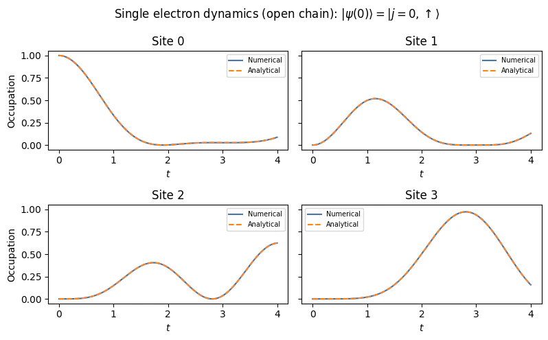
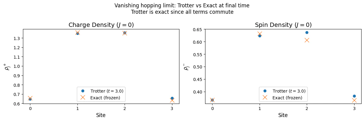
Vanishing hopping limit
The other extreme is obtained when the onsite interactions is much larger than the hopping constant. In this regime interaction dominate the physics and supress hopping between adjacent sites, allowing us to take . The FH Hamiltonian then becomes a sum of local commuting terms, diagonal in the Fock basis (eigenstates of the number operators ). The Hamiltonian reduces to where n.h denotes “no hopping”. As a consequence the local number operators are a constant of motion , and we expect the charges to freeze in time. Since all terms in commute with one another, i.e., for all , the first-order Trotter decomposition is exact: This means the Trotter circuit reproduces the exact time evolution with no approximation error, regardless of the step size . To verify this, we prepare an initial state that is not an eigenstate of — specifically, the ground state of the non-interacting Hamiltonian with an attractive potential (a Slater determinant with non-uniform charge distribution). We then compare the Trotter dynamics with the exact analytical prediction: frozen charge and spin densities.Numerical Evaluation
Output: