Hamiltonian Simulation with Generalized Quantum Signal Processing (GQSP)

View on GitHub

Open this notebook in GitHub to run it yourself

Simulating physical and chemical systems was among the original motivations for quantum computing, as first envisioned by Richard Feynman in 1982, and remains one of its most impactful applications. Time-independent Hamiltonian simulation refers to the task of approximately implementing the unitary evolution operator $e^{-iHt}$ for a Hermitian matrix $H$ . When access to the Hamiltonian is provided via block-encoding, this can be realized by applying an appropriate polynomial transformation within a desired precision $\epsilon$ . Generalized Quantum Signal Processing (GQSP) [1] achieves this by applying a Laurent polynomial $P(W)$ to the walk operator $W$ of the block-encoded Hamiltonian. The polynomial coefficients are derived from the Jacobi–Anger expansion (Eq. (1): $e^{it\cos(x)} = \sum_k i^k J_k(t)\,e^{ikx}$ ). GQSP requires only one auxiliary qubit and eliminates the need for amplitude amplification.

Input: A Hermitian operator $H$ given through a block-encoding unitary $U_H$ with scaling factor $\alpha \ge \|H\|$ , evolution time $t$ , and target error $\epsilon$ .

Output: A unitary $U$ approximating $e^{-iHt}$ , with $\|U - e^{-iHt}\| < \epsilon$ .

Complexity: $O\!\left(\alpha t + \frac{\log \epsilon^{-1}}{\log\!\left(e + \log(\epsilon^{-1}) / \alpha t\right)}\right)$ calls to the block-encoding, using one auxiliary qubit and a classical preprocessing step to compute the GQSP rotation angles.
Keywords: Hamiltonian Simulation, Block Encoding, Generalized Quantum Signal Processing, GQSP, Walk Operator, Oracle/Query complexity.

A block-encoded Hamiltonian refers to its embedding within a larger unitary matrix. Definition: A

(s, m, \epsilon)

-encoding of a

2^n\times 2^n

matrix

A

refers to completing it into a

2^{n+m}\times 2^{n+m}

unitary matrix

U_{(s,m,\epsilon)-A}

U_{(s,m,\epsilon)-A} = \begin{pmatrix} A/s & * \\ * & * \end{pmatrix},

with functional error

\left|\left|\left(U_{(s,m,\epsilon)-A}\right)_{0:2^n-1,0:2^n-1}-A/s \right|\right|\leq \epsilon

. Here

s

is a scaling factor that ensures the overall operator is unitary,

m

is the number of auxiliary (block) qubits, and

\epsilon

is the encoding error. This notebook assumes basic knowledge of Linear Combination of Unitaries (LCU); see the LCU tutorial for background. The GQSP approach implements polynomials on unitary operators. For Hamiltonian evolution, given an exact

(s, m, 0)

-encoding of the Hamiltonian (denoting

U_H \equiv U_{(s,m,0)-H}

), we define the Szegedy quantum walk operator [2]

W \equiv \Pi_{|0\rangle_m}\, U_H

, where

\Pi_{|0\rangle_m}

reflects about the

|0\rangle

state of the block variable. The walk operator

W

is unitary, with eigenvalues

z = e^{\pm i\arccos(\lambda/s)}

, where

\lambda

are the Hamiltonian eigenvalues. By the Jacobi–Anger expansion (Eq. (1)), the polynomial approximating

e^{-ist\cos(x)}

as a Laurent series in

z = e^{ix}

gives

P(z) \approx e^{-i\lambda t}

on the eigenvalue

z = e^{i\arccos(\lambda/s)}

(since

\cos(x) = \lambda/s

) — the desired time-evolution phase. Applying

P(W)

via GQSP therefore gives approximately

e^{-iHt}

in the block. GQSP computes a set of single-qubit rotation angles

\{\phi_k\}

such that the resulting circuit block-encodes the desired polynomial:

\mathrm{GQSP}(W) \approx U_{(1,\,m+1,\,\epsilon)-e^{-iHt}} = \begin{pmatrix} e^{-iHt} & * \\ * & * \end{pmatrix}.

(In practice, our prefactor is slightly different,

\beta^{-1}

with

\beta = 0.9999

which ensures numerical stability of the classical angle computation). Compared the the QSVT approach for Hamiltonian simulation, the GQSP method uses only one extra block qubit, and requires no amplitude amplification. However, it includes controlled operations on the block-encoding unitary.

This notebook demonstrates Hamiltonian simulation using the GQSP method.For the other approaches, see the companion notebooks on QSVT and Qubitization.For a side-by-side comparison of all three methods, see the table at the end of this notebook.

Preliminaries

Setting a Specific Hamiltonian to Evolve

We set some specific hyperparameters for our problem. We use a simple Hamiltonian given as a sum of Pauli strings, and the lcu_pauli function to block-encode it via the Linear Combination of Unitaries (LCU) technique:

H = \sum_{i} \alpha_i U_i, \qquad U_{(\bar{\alpha},m,0)-H} = \begin{pmatrix} H/\bar{\alpha} & * \\ * & * \end{pmatrix}, \qquad \bar{\alpha} = \sum_i |\alpha_i|.

To treat different problems with the same algorithm, simply change theses hyperparameters.

import time

import matplotlib.pyplot as plt
import numpy as np
import scipy

from classiq import *

EVOLUTION_TIME = 22
EPS = 1e-7

HAMILTONIAN = (
    0.4 * Pauli.I(0)
    + 0.1 * Pauli.Z(1)
    + 0.05 * Pauli.X(0) * Pauli.X(1)
    + 0.2 * Pauli.Z(0) * Pauli.Z(1)
)
print(f"The Hamiltonian to evolve: {HAMILTONIAN}")

Output:

The Hamiltonian to evolve: 0.4 + 0.05*Pauli.X(0)*Pauli.X(1) + 0.2*Pauli.Z(0)*Pauli.Z(1) + 0.1*Pauli.Z(1)
  

Next, we define the block-encoding quantum function, and a Quantum Struct for its variable.

data_size = HAMILTONIAN.num_qubits
block_size = (
    (len(HAMILTONIAN.terms) - 1).bit_length() if len(HAMILTONIAN.terms) != 1 else 1
)
BE_SCALING = np.sum(
    np.abs([term.coefficient for term in HAMILTONIAN.terms])
)  # scaling for LCU of Paulis

print(f"Block size: {block_size}")
print(f"Block-encoding scaling factor: {BE_SCALING}")


class BlockEncodedState(QStruct):
    data: QNum[data_size]
    block: QNum[block_size]


@qfunc
def be_hamiltonian(state: BlockEncodedState):
    lcu_pauli(HAMILTONIAN * (1 / BE_SCALING), state.data, state.block)

Output:

Block size: 2
  Block-encoding scaling factor: 0.75
  

Finally, we set the initial state to evolve and calculate classically the expected evolved state for verifying the quantum methods.

state_to_evolve = np.random.rand(2**data_size)
state_to_evolve = (state_to_evolve / np.linalg.norm(state_to_evolve)).tolist()
matrix = pauli_operator_to_matrix(HAMILTONIAN)
expected_state = scipy.linalg.expm(-1j * matrix * EVOLUTION_TIME) @ state_to_evolve

Setting Up a Statevector Simulator

Working with block-encoding typically requires post-selection of the block variable being at state

|0\rangle

. The success of this process can be amplified via Oblivious Amplitude Amplification. In this notebook, instead, we use a statevector simulator and project the result. We import two utility functions from hamiltonian_simulation_utils:

get_projected_state_vector: extracts the post-selected statevector from the execution results.
compare_quantum_classical_states: aligns the global phase and computes the overlap with the classically computed reference.

from hamiltonian_simulation_utils import (
    compare_quantum_classical_states,
    get_projected_state_vector,
)

execution_preferences = ExecutionPreferences(
    num_shots=1,
    backend_preferences=ClassiqBackendPreferences(
        backend_name=ClassiqSimulatorBackendNames.SIMULATOR_STATEVECTOR
    ),
)

The Jacobi–Anger Expansion

The polynomial approximation of the time evolution relies on the Jacobi–Anger expansion. For GQSP, we use the complex exponential form

e^{it\cos(x)} = \sum_k i^k J_k(t)\,e^{ikx}

, implemented via poly_jacobi_anger_exp_cos. We then compute the GQSP rotation angles from this polynomial using gqsp_phases.

from classiq.applications.qsp.qsp import (
    gqsp_phases,
    poly_jacobi_anger_degree,
    poly_jacobi_anger_exp_cos,
)

GQSP_SCALE = 0.9999
t0 = time.perf_counter()
gqsp_degree = poly_jacobi_anger_degree(EPS, EVOLUTION_TIME * BE_SCALING)

jacobi_anger_poly_expcos = GQSP_SCALE * poly_jacobi_anger_exp_cos(
    gqsp_degree, -EVOLUTION_TIME * BE_SCALING
)
jacobi_anger_phases_expcos = gqsp_phases(jacobi_anger_poly_expcos)
classical_preprocess_time_gqsp = time.perf_counter() - t0
print(f"GQSP polynomial degree: {gqsp_degree}")
print(f"Classical preprocessing time: {classical_preprocess_time_gqsp:.3f} s")

Output:

GQSP polynomial degree: 33
  Classical preprocessing time: 2.932 s
  

The Walk Operator

Note: The current implementation assumes that the block-encoding unitary $U_H$ is also Hermitian. For the non-Hermitian generalization, see the Technical Notes.

Given the block-encoding

U_{(s,m,0)-H}

, we define the Szegedy quantum walk operator [2]:

W \equiv \Pi_{|0\rangle_m}\, U_{(s,m,0)-H},

where

\Pi_{|0\rangle_m}

is a reflection about the

|0\rangle

state of the block variable. As mentioned above, it has the key property that its spectrum is directly tied to the Hamiltonian’s eigenvalues:

\text{eigenvalues: } e^{\pm i \arccos(\lambda/s)}, \quad \text{eigenvectors: } |\varphi^{\pm}_{\lambda}\rangle \equiv \frac{1}{\sqrt{2}}\left(|v_{\lambda}\rangle|0\rangle_m \pm i|\perp_{\lambda}\rangle\right),

where

|v_\lambda\rangle

is an eigenstate of

H

with eigenvalue

\lambda

from classiq.qmod.symbolic import pi


@qfunc
def my_reflect_about_zero(qba: QNum):
    control(qba == 0, lambda: phase(pi))
    phase(pi)


@qfunc
def walk_operator(
    be_qfunc: QCallable[BlockEncodedState], state: BlockEncodedState
) -> None:
    be_qfunc(state)
    my_reflect_about_zero(state.block)

Verifying the Block-Encoding

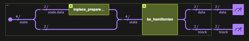
As a sanity check before the main algorithm, we verify the Hamiltonian block-encoding: we apply

U_H

on the initial state and check that the post-selected result matches

(H/\bar{\alpha})|\psi\rangle

as expected.

@qfunc
def main(data: Output[QNum[data_size]], block: Output[QNum[block_size]]):
    state = BlockEncodedState()
    allocate(state)

    inplace_prepare_amplitudes(state_to_evolve, 0.0, state.data)
    be_hamiltonian(state)
    bind(state, [data, block])


qprog_be = synthesize(main)
show(qprog_be)

Output:

Quantum program link: https://platform.classiq.io/circuit/3D33qBTW7qLuxJGlgJOoBiBBhwH
  

TOLERANCE = 1e-9
with ExecutionSession(qprog_be, execution_preferences=execution_preferences) as es:
    res_be = es.sample()

state_result_be = get_projected_state_vector(res_be)
expected_state_be = matrix @ state_to_evolve

renormalized_be, overlap_be = compare_quantum_classical_states(
    expected_state_be, state_result_be, BE_SCALING
)
print("Expected state:", expected_state_be)
print("Resulting state after rescaling:", renormalized_be)
assert np.isclose(overlap_be, 1, TOLERANCE)
print("=" * 40)
print(f"Fidelity is 1 (with {TOLERANCE} tolerance)")

Output:

Expected state: [0.62080558+0.j 0.09074939+0.j 0.04500028+0.j 0.18596617+0.j]
  Resulting state after rescaling: [0.62080558+2.44087822e-18j 0.09074939-9.63604777e-17j
   0.04500028-2.02041677e-16j 0.18596617-1.14021062e-16j]
  ========================================
  Fidelity is 1 (with 1e-09 tolerance)
  

Implementation

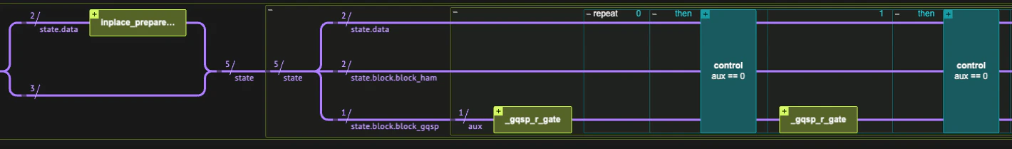
We define a Quantum Struct for the GQSP block-encoding. The GQSP method adds one block qubit (block_gqsp) to the Hamiltonian block variable (block_ham). The data variable follows that of the Hamiltonian encoding. Applying GQSP requires a negative power of the walk operator, since the approximating polynomial

P(z)

is a Laurent polynomial that includes negative powers of

z

(corresponding to

W^{-1}

). This is handled by the negative_power parameter.

class GQSPBlock(QStruct):
    block_ham: QNum[block_size]
    block_gqsp: QBit


class GQSPState(QStruct):
    data: QNum[data_size]
    block: GQSPBlock


@qfunc
def gqsp_hamiltonian_evolution(
    be_qfunc: QCallable[BlockEncodedState],
    state: GQSPState,
):
    gqsp(
        u=lambda: walk_operator(be_qfunc, [state.data, state.block.block_ham]),
        aux=state.block.block_gqsp,
        phases=jacobi_anger_phases_expcos,
        negative_power=gqsp_degree,
    )

The code in the rest of this section builds a model that applies the gqsp_hamiltonian_evolution function on the randomly prepared vector, synthesizes it, executes the resulting quantum program, and verifies the results.

@qfunc
def main(data: Output[QNum[data_size]], block: Output[QNum[block_size + 1]]):
    state = GQSPState()
    allocate(state)

    inplace_prepare_amplitudes(state_to_evolve, 0.0, state.data)
    gqsp_hamiltonian_evolution(be_hamiltonian, state)
    bind(state, [data, block])


qprog_gqsp = synthesize(main)
show(qprog_gqsp)

Output:

Quantum program link: https://platform.classiq.io/circuit/3D33t06StqkU0O0rBRxsTEFVZF4
  

with ExecutionSession(qprog_gqsp, execution_preferences) as es:
    result_gqsp = es.sample()

state_result_gqsp = get_projected_state_vector(result_gqsp)
exp_scaling_factor_gqsp = 1 / GQSP_SCALE

renormalized_state_gqsp, overlap_gqsp = compare_quantum_classical_states(
    expected_state, state_result_gqsp, exp_scaling_factor_gqsp
)
print("Expected state:", expected_state)
print("Resulting state after rescaling:", renormalized_state_gqsp)
assert np.linalg.norm(renormalized_state_gqsp - expected_state) < EPS
print("=" * 40)
print("Overlap between expected and resulting state:", overlap_gqsp)

Output:

Expected state: [-0.87895119-0.0601642j   0.2797734 -0.11212048j -0.03050629-0.27574903j
   -0.22787636+0.06391499j]
  Resulting state after rescaling: [-0.87895119-0.0601642j   0.27977341-0.11212048j -0.03050629-0.27574903j
   -0.22787636+0.06391499j]
  ========================================
  Overlap between expected and resulting state: 1.0000000000000002
  

References

[1]: Motlagh, D., and Wiebe, N. Generalized quantum signal processing. PRX Quantum 5, 020368 (2024). [2]: Szegedy, M. Quantum speed-up of Markov chain based algorithms. In 45th Annual IEEE Symposium on Foundations of Computer Science, pp. 32–41 (2004). [3]: Lin, L. Lecture notes on quantum algorithms for scientific computation. arXiv:2201.08309 [quant-ph] (2022).

Technical Notes

Generalizing to Non-Hermitian Block-Encoding Unitaries

The current implementation assumes that the block-encoding unitary

U_H

is also Hermitian. This assumption underlies the walk operator’s spectral properties. For a non-Hermitian block-encoding unitary, an analogous walk operator can be defined as

\tilde{W} \equiv U_H^T \Pi_{|0\rangle_m} U_H \Pi_{|0\rangle_m}

, which satisfies equivalent spectral properties. See Section 7.4 in Ref. [3] for details.

Comparison with Other Methods

Method	extra block qubits	Controlled $U_H$ ?	Amplitude amplification?	Classical preprocessing
GQSP	1	Yes	No	Angle computation
QSVT	2	No	Yes (for a factor of 2)	Angle computation
Qubitization	$O(\log d)$	Yes	Yes (for the sum of Cheb. coefficients)	None

All three methods share the same asymptotic query complexity. Differences in the table reflect the detailed implementation of this specific example.

Algorithms

Applications

Functions

Tutorials

Hamiltonian Simulation with Generalized Quantum Signal Processing (GQSP)

View on GitHub

Preliminaries

Setting a Specific Hamiltonian to Evolve

Setting Up a Statevector Simulator

The Jacobi–Anger Expansion

The Walk Operator

Verifying the Block-Encoding

Implementation

References

Technical Notes

Generalizing to Non-Hermitian Block-Encoding Unitaries

Comparison with Other Methods

Algorithms

Applications

Functions

Tutorials

Documentation Index

View on GitHub

​Preliminaries

​

​Setting a Specific Hamiltonian to Evolve

​

​Setting Up a Statevector Simulator

​

​The Jacobi–Anger Expansion

​

​The Walk Operator

​

​Verifying the Block-Encoding

​Implementation

​References

​Technical Notes

​

​Generalizing to Non-Hermitian Block-Encoding Unitaries

​

​Comparison with Other Methods

Preliminaries

Setting a Specific Hamiltonian to Evolve

Setting Up a Statevector Simulator

The Jacobi–Anger Expansion

The Walk Operator

Verifying the Block-Encoding

Implementation

References

Technical Notes

Generalizing to Non-Hermitian Block-Encoding Unitaries

Comparison with Other Methods