Hamiltonian Simulation with Quantum Singular Value Transformation (QSVT)

View on GitHub

Open this notebook in GitHub to run it yourself

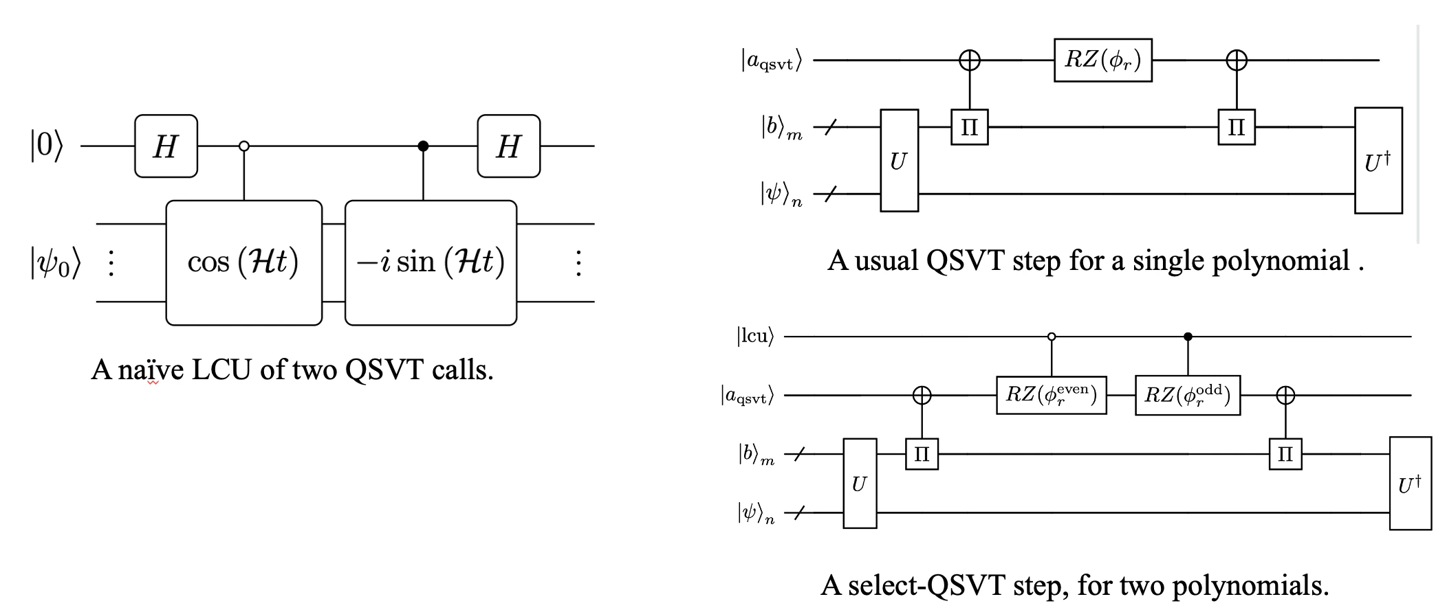
Simulating physical and chemical systems was among the original motivations for quantum computing, as first envisioned by Richard Feynman in 1982, and remains one of its most impactful applications. Time-independent Hamiltonian simulation refers to the task of approximately implementing the unitary evolution operator $e^{-iHt}$ for a Hermitian matrix $H$ . When access to the Hamiltonian is provided via block-encoding, this can be realized by applying an appropriate polynomial transformation within a desired precision $\epsilon$ . Quantum Singular Value Transformation (QSVT) [1] achieves Hamiltonian simulation by exploiting the decomposition $e^{-iHt} = \cos(Ht) - i\sin(Ht)$ . Two QSVT blocks, one for the even polynomial $\cos(xt)$ and one for the odd polynomial $\sin(xt)$ (both approximated via the Jacobi–Anger expansion, Eqs. (3)-(4)), are combined via LCU. Unlike GQSP and Qubitization, QSVT operates directly on the block-encoding without requiring a walk operator or controlled block-encoding calls, using only two auxiliary qubits.

Input: A Hermitian operator $H$ given through a block-encoding unitary $U_H$ with scaling factor $\alpha \ge \|H\|$ , evolution time $t$ , and target error $\epsilon$ .

Output: A unitary $U$ approximating $e^{-iHt}$ , with $\|U - e^{-iHt}\| < \epsilon$ .

Complexity: $O\!\left(\alpha t + \frac{\log \epsilon^{-1}}{\log\!\left(e + \log(\epsilon^{-1}) / \alpha t\right)}\right)$ calls to the block-encoding, using two auxiliary qubits. No controlled block-encoding calls required. Requires classical preprocessing to compute QSVT rotation angles.
Keywords: Hamiltonian Simulation, Block Encoding, Quantum Singular Value Transformation, QSVT, Quantum Signal Processing, LCU, Oracle/Query complexity.

A block-encoded Hamiltonian refers to its embedding within a larger unitary matrix. Definition: A

(s, m, \epsilon)

-encoding of a

2^n\times 2^n

matrix

A

refers to completing it into a

2^{n+m}\times 2^{n+m}

unitary matrix

U_{(s,m,\epsilon)-A}

U_{(s,m,\epsilon)-A} = \begin{pmatrix} A/s & * \\ * & * \end{pmatrix},

with functional error

\left|\left|\left(U_{(s,m,\epsilon)-A}\right)_{0:2^n-1,0:2^n-1}-A/s \right|\right|\leq \epsilon

. Here

s

is a scaling factor that ensures the overall operator is unitary,

m

is the number of auxiliary (block) qubits, and

\epsilon

is the encoding error. This notebook assumes basic knowledge of Linear Combination of Unitaries (LCU) and the PREPARE–SELECT implementation; see the LCU tutorial for background. We assume an exact

(s, m, 0)

-encoding of the Hamiltonian as input. The QSVT method outputs an approximated block-encoding of its time evolution:

U_{(s,m,0)-H} \;\rightarrow\; U_{(2,\,m+2,\,\epsilon)-\exp(-iHt)} = \begin{pmatrix} \exp(-iHt)/2 & * \\ * & * \end{pmatrix}.

This is achieved by implementing a block-encoding for the polynomial approximation

P(H)\approx \frac{1}{\tilde{s}}e^{-iHt}

. To recover the exact unitary

e^{-iHt}

one would apply amplitude amplification to drive the prefactor

1/2\rightarrow 1

; here we instead employ projected statevector simulation. QSVT is a general method for implementing polynomial singular value transformation of block-encoded matrices, where each polynomial must have a well-defined parity (even or odd). The transformation is based on Quantum Signal Processing (QSP), achieved by a series of qubit rotations. In the case of general polynomial transformation, as in Hamiltonian simulation

e^{-iHt} = \cos(Ht) - i\sin(Ht)

, one can apply two polynomial transformations, one for the even polynomial

\cos(xt)

and one for the odd polynomial

\sin(xt)

, combined via Linear Combination of Unitaries (LCU). The two QSVT circuits are combined using the qsvt_lcu function, which implements an optimized select operation that interleaves the rotations of both polynomials within a single QSVT traversal. The overall result is a

(2,\,m+2,\,\epsilon)

-block-encoding of

e^{-iHt}

, where one block qubit comes from the QSVT and the second one, as well as the

1/2

prefactor, originates from the LCU. (In practice, our prefactor is slightly different,

2\beta^{-1}

with

\beta = 0.9999

which ensures numerical stability of the classical angle computation).

This notebook demonstrates Hamiltonian simulation using the QSVT method.For the other approaches, see the companion notebooks on GQSP and Qubitization.For a side-by-side comparison of all three methods, see the table at the end of this notebook.

Preliminaries

Setting a Specific Hamiltonian to Evolve

We set some specific hyperparameters for our problem. We use a simple Hamiltonian given as a sum of Pauli strings, and the lcu_pauli function to block-encode it via the Linear Combination of Unitaries (LCU) technique:

H = \sum_{i} \alpha_i U_i, \qquad U_{(\bar{\alpha},m,0)-H} = \begin{pmatrix} H/\bar{\alpha} & * \\ * & * \end{pmatrix}, \qquad \bar{\alpha} = \sum_i |\alpha_i|.

To treat different problems with the same algorithm, simply change theses hyperparameters.

import time

import matplotlib.pyplot as plt
import numpy as np
import scipy

from classiq import *

EVOLUTION_TIME = 22
EPS = 1e-7

HAMILTONIAN = (
    0.4 * Pauli.I(0)
    + 0.1 * Pauli.Z(1)
    + 0.05 * Pauli.X(0) * Pauli.X(1)
    + 0.2 * Pauli.Z(0) * Pauli.Z(1)
)
print(f"The Hamiltonian to evolve: {HAMILTONIAN}")

Output:

The Hamiltonian to evolve: 0.4 + 0.05*Pauli.X(0)*Pauli.X(1) + 0.2*Pauli.Z(0)*Pauli.Z(1) + 0.1*Pauli.Z(1)
  

Next, we define the block-encoding quantum function, and a Quantum Struct for its variable.

data_size = HAMILTONIAN.num_qubits
block_size = (
    (len(HAMILTONIAN.terms) - 1).bit_length() if len(HAMILTONIAN.terms) != 1 else 1
)
BE_SCALING = np.sum(
    np.abs([term.coefficient for term in HAMILTONIAN.terms])
)  # scaling for LCU of Paulis

print(f"Block size: {block_size}")
print(f"Block-encoding scaling factor: {BE_SCALING}")


class BlockEncodedState(QStruct):
    data: QNum[data_size]
    block: QNum[block_size]


@qfunc
def be_hamiltonian(state: BlockEncodedState):
    lcu_pauli(HAMILTONIAN * (1 / BE_SCALING), state.data, state.block)

Output:

Block size: 2
  Block-encoding scaling factor: 0.75
  

Finally, we set the initial state to evolve and calculate classically the expected evolved state for verifying the quantum method.

state_to_evolve = np.random.rand(2**data_size)
state_to_evolve = (state_to_evolve / np.linalg.norm(state_to_evolve)).tolist()
matrix = pauli_operator_to_matrix(HAMILTONIAN)
expected_state = scipy.linalg.expm(-1j * matrix * EVOLUTION_TIME) @ state_to_evolve

Setting Up a Statevector Simulator

Working with block-encoding typically requires post-selection of the block variable being at state

|0\rangle

. The success of this process can be amplified via Oblivious Amplitude Amplification. In this notebook, instead, we use a statevector simulator and project the result. We import two utility functions from hamiltonian_simulation_utils:

get_projected_state_vector: extracts the post-selected statevector from the execution results.
compare_quantum_classical_states: aligns the global phase and computes the overlap with the classically computed reference.

from hamiltonian_simulation_utils import (
    compare_quantum_classical_states,
    get_projected_state_vector,
)

execution_preferences = ExecutionPreferences(
    num_shots=1,
    backend_preferences=ClassiqBackendPreferences(
        backend_name=ClassiqSimulatorBackendNames.SIMULATOR_STATEVECTOR
    ),
)

The Jacobi–Anger Expansion

The polynomial approximation of the time evolution relies on the Jacobi–Anger expansion. For QSVT, we use the real Chebyshev forms

\cos(xt)

and

\sin(xt)

(Eqs. (3)–(4)), computed via poly_jacobi_anger_cos and poly_jacobi_anger_sin. From these, we derive the QSVT rotation angles using qsvt_phases.

from classiq.applications.qsp import qsvt_phases
from classiq.applications.qsp.qsp import (
    poly_jacobi_anger_cos,
    poly_jacobi_anger_degree,
    poly_jacobi_anger_sin,
)

t0 = time.perf_counter()

qsvt_degree = poly_jacobi_anger_degree(EPS, EVOLUTION_TIME * BE_SCALING)
COS_SCALE = SIN_SCALE = 0.9999
poly_even = COS_SCALE * poly_jacobi_anger_cos(qsvt_degree, EVOLUTION_TIME * BE_SCALING)
phases_cos = qsvt_phases(poly_even)

poly_odd = SIN_SCALE * poly_jacobi_anger_sin(qsvt_degree, EVOLUTION_TIME * BE_SCALING)
phases_sin = qsvt_phases(poly_odd)

classical_preprocess_time_qsvt = time.perf_counter() - t0
print(f"QSVT polynomial degree: {qsvt_degree}")
print(f"Classical preprocessing time: {classical_preprocess_time_qsvt:.3f} s")

assert np.abs(len(phases_sin) - len(phases_cos)) <= 1

Output:

QSVT polynomial degree: 33
  Classical preprocessing time: 2.870 s
  

Verifying the Block-Encoding

As a sanity check before the main algorithm, we verify the Hamiltonian block-encoding: we apply

U_H

on the initial state and check that the post-selected result matches

(H/\bar{\alpha})|\psi\rangle

as expected.

@qfunc
def main(data: Output[QNum[data_size]], block: Output[QNum[block_size]]):
    state = BlockEncodedState()
    allocate(state)

    inplace_prepare_amplitudes(state_to_evolve, 0.0, state.data)
    be_hamiltonian(state)
    bind(state, [data, block])


qprog_be = synthesize(main)
show(qprog_be)

Output:

Quantum program link: https://platform.classiq.io/circuit/3D33xB4bjrs7vhRP4pqVIiFuFPy
  

TOLERANCE = 1e-9
with ExecutionSession(qprog_be, execution_preferences=execution_preferences) as es:
    res_be = es.sample()

state_result_be = get_projected_state_vector(res_be)
expected_state_be = matrix @ state_to_evolve

renormalized_be, overlap_be = compare_quantum_classical_states(
    expected_state_be, state_result_be, BE_SCALING
)
print("Expected state:", expected_state_be)
print("Resulting state after rescaling:", renormalized_be)
assert np.isclose(overlap_be, 1, TOLERANCE)
print("=" * 40)
print(f"Fidelity is 1 (with {TOLERANCE} tolerance)")

Output:

Expected state: [0.01550541+0.j 0.27717585+0.j 0.09124952+0.j 0.11147152+0.j]
  Resulting state after rescaling: [0.01550541-3.18016883e-18j 0.27717585-3.83523176e-15j
   0.09124952-1.32318732e-15j 0.11147152-1.60360148e-15j]
  ========================================
  Fidelity is 1 (with 1e-09 tolerance)
  

Implementation

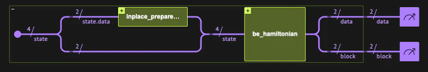
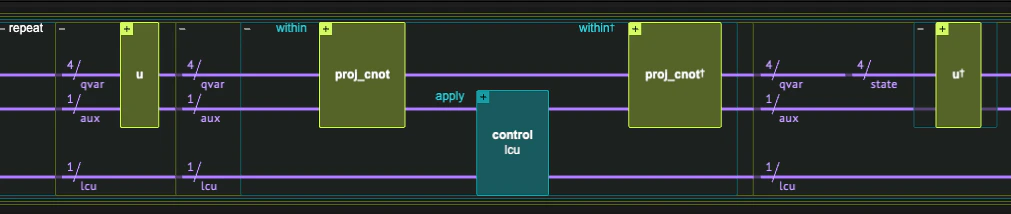
We define Quantum Structs for the QSVT block-encoding. Two block qubits are used: one for the QSVT signal processing (block_qsvt) and one for the LCU, selecting between odd and even polynomials (block_lcu). These are added to the block variable of the Hamiltonian encoding. The qsvt_hamiltonian_evolution function uses prepare_select with the qsvt_lcu as the select operation. The LCU coefficients

(1/2, -i/2)

implement

\frac{1}{2}(\cos(Ht) - i\sin(Ht)) = \frac{1}{2}e^{-iHt}

. The projector_cnot function implements the QSVT projector onto the

|0\rangle

state of the Hamiltonian block variable.

class QSVTBlock(QStruct):
    block_ham: QNum[block_size]
    block_qsvt: QBit
    block_lcu: QBit


class QSVTState(QStruct):
    data: QNum[data_size]
    block: QSVTBlock


@qfunc
def qsvt_hamiltonian_evolution(
    phases_cos: list[float],
    phases_sin: list[float],
    be_qfunc: QCallable[BlockEncodedState],
    state: QSVTState,
):
    def projector_cnot(q: QBit):
        q ^= state.block.block_ham == 0

    prepare_select(
        coefficients=[1 / 2, -1j / 2],
        select=lambda block_lcu: qsvt_lcu(
            phases_cos,
            phases_sin,
            projector_cnot,
            projector_cnot,
            lambda: be_qfunc([state.data, state.block.block_ham]),
            state.block.block_qsvt,
            block_lcu,
        ),
        block=state.block.block_lcu,
    )

The code in the rest of this section builds a model that applies the qsvt_hamiltonian_evolution function on the randomly prepared vector

(\vec{\psi},\vec{0})

, synthesizes it, executes the resulting quantum program, and verifies the results.

@qfunc
def main(data: Output[QNum[data_size]], block: Output[QNum[block_size + 2]]):
    state = QSVTState()
    allocate(state)
    inplace_prepare_amplitudes(state_to_evolve, 0.0, state.data)
    qsvt_hamiltonian_evolution(phases_cos, phases_sin, be_hamiltonian, state)
    bind(state, [data, block])


qprog_qsvt = synthesize(main, constraints=Constraints(optimization_parameter="width"))
show(qprog_qsvt)

Output:

Quantum program link: https://platform.classiq.io/circuit/3D341fNgiDKLoX6iTNuqKHwx7yH
  

with ExecutionSession(qprog_qsvt, execution_preferences) as es:
    results_qsvt = es.sample()

state_result_qsvt = get_projected_state_vector(results_qsvt)
exp_scaling_factor_qsvt = 2 * (1 / COS_SCALE)

renormalized_state_qsvt, overlap_qsvt = compare_quantum_classical_states(
    expected_state, state_result_qsvt, exp_scaling_factor_qsvt
)
print("Expected state:", expected_state)
print("Resulting state after rescaling:", renormalized_state_qsvt)
assert np.linalg.norm(renormalized_state_qsvt - expected_state) < EPS
print("=" * 40)
print("Overlap between expected and resulting state:", overlap_qsvt)

Output:

Expected state: [-0.04311848-0.05046671j  0.7844373 -0.43360491j  0.07945592-0.37532381j
   -0.06593688+0.20176705j]
  Resulting state after rescaling: [-0.04311848-0.05046671j  0.7844373 -0.43360491j  0.07945593-0.37532381j
   -0.06593688+0.20176705j]
  ========================================
  Overlap between expected and resulting state: 1.0
  

References

[1]: Martyn, J. M., Rossi, Z. M., Tan, A. K., & Chuang, I. L. Grand unification of quantum algorithms. PRX Quantum 2, 040203 (2021).

Technical Notes

Comparison with Other Methods

Method	extra block qubits	Controlled $U_H$ ?	Amplitude amplification?	Classical preprocessing
GQSP	1	Yes	No	Angle computation
QSVT	2	No	Yes (for a factor of 2)	Angle computation
Qubitization	$O(\log d)$	Yes	Yes (for the sum of Cheb. coefficients)	None

All three methods share the same asymptotic query complexity. Differences in the table reflect the detailed implementation of this specific example.

Algorithms

Applications

Functions

Tutorials

Hamiltonian Simulation with Quantum Singular Value Transformation (QSVT)

View on GitHub

Preliminaries

Setting a Specific Hamiltonian to Evolve

Setting Up a Statevector Simulator

The Jacobi–Anger Expansion

Verifying the Block-Encoding

Implementation

References

Technical Notes

Comparison with Other Methods

Algorithms

Applications

Functions

Tutorials

Documentation Index

View on GitHub

​Preliminaries

​

​Setting a Specific Hamiltonian to Evolve

​

​Setting Up a Statevector Simulator

​

​The Jacobi–Anger Expansion

​

​Verifying the Block-Encoding

​Implementation

​References

​Technical Notes

​

​Comparison with Other Methods

Preliminaries

Setting a Specific Hamiltonian to Evolve

Setting Up a Statevector Simulator

The Jacobi–Anger Expansion

Verifying the Block-Encoding

Implementation

References

Technical Notes

Comparison with Other Methods