

Documentation Index
Fetch the complete documentation index at: https://prod-mint.classiq.io/llms.txt
Use this file to discover all available pages before exploring further.
View on GitHub
Open this notebook in GitHub to run it yourself
- Hamiltonian Simulation with GQSP
- Hamiltonian Simulation with QSVT
- Hamiltonian Simulation with Qubitization
The Expansion
The most general form of the Jacobi–Anger expansion [1] gives: from which we can derive Chebyshev polynomial series for the real-valued functions: where is the Bessel function of the first kind of order , and is the Chebyshev polynomial of order . Eq. (1) is directly used in the GQSP method (applied to the walk operator). Eqs. (3)–(4) are used by both the QSVT method and the Qubitization method.Truncation and Error Bound
The infinite series in Eqs. (3) and (4) can be truncated at degree , giving polynomial approximations of and . The required degree for a target approximation error and evolution time is: This scaling, linear in and logarithmic in , is optimal: it matches the quantum query complexity lower bound for Hamiltonian simulation [2]. This is one of the key reasons the block-encoding family of algorithms is asymptotically optimal. Classiq’s QSP application includes all 5 formulas above. Next we demonstrate the approximation for a given evolution time and error , for the expansion of the function and (Eqs. (3) and (4) above).Output:
Approximation Quality
We can visually inspect the approximation quality for and :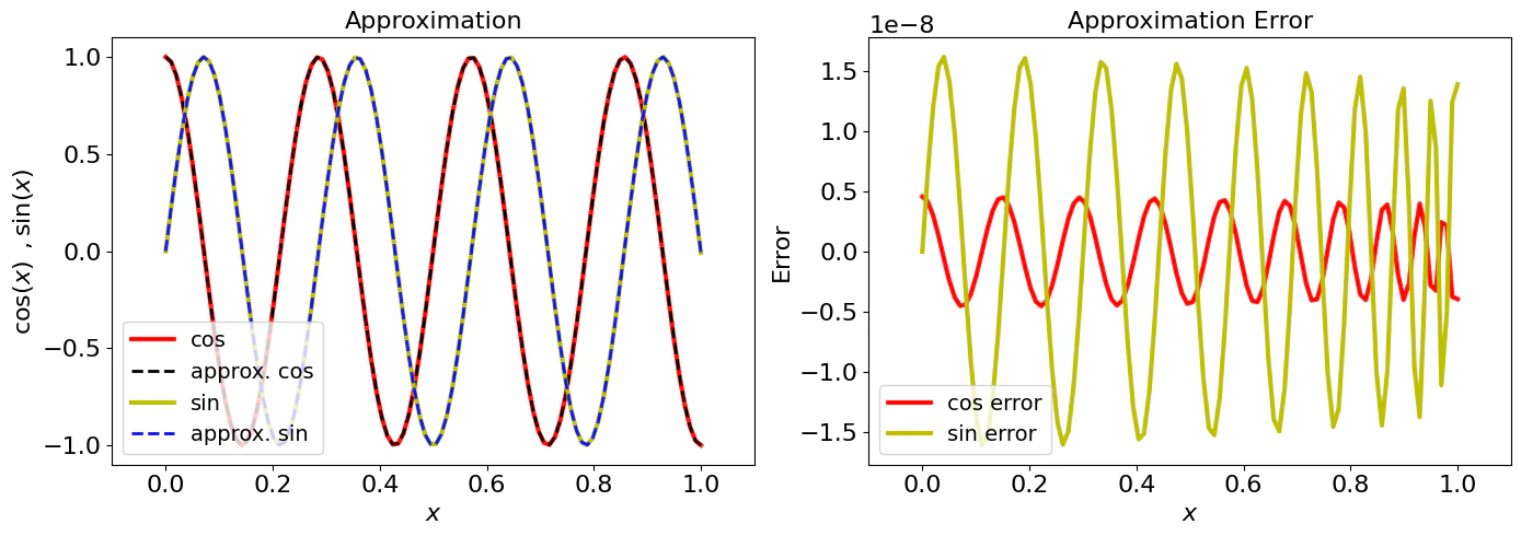
See Also
This expansion is the mathematical foundation used by each of the three Hamiltonian simulation notebooks in this directory:- Hamiltonian Simulation with GQSP — applies Eq. (1) as a Laurent polynomial in the walk operator .
- Hamiltonian Simulation with QSVT — applies Eqs. (3)–(4) as two separate QSVT polynomial transformations, combined via LCU.
- Hamiltonian Simulation with Qubitization — applies Eqs. (3)–(4) directly as Chebyshev coefficients in an LCU of walk operator powers.