Hamiltonian Simulation with Qubitization (Chebyshev LCU)

View on GitHub

Open this notebook in GitHub to run it yourself

Simulating physical and chemical systems was among the original motivations for quantum computing, as first envisioned by Richard Feynman in 1982, and remains one of its most impactful applications. Time-independent Hamiltonian simulation refers to the task of approximately implementing the unitary evolution operator $e^{-iHt}$ for a Hermitian matrix $H$ . When access to the Hamiltonian is provided via block-encoding, this can be realized by applying an appropriate polynomial transformation within a desired precision $\epsilon$ . Qubitization [1] achieves Hamiltonian simulation by combining the Jacobi–Anger expansion with the Linear Combination of Unitaries (LCU) technique, exploiting the fact that powers of the walk operator directly implement Chebyshev polynomial block-encodings. This approach is entirely constructive- it requires no classical preprocessing for rotation angles, but uses more ancilla qubits ( $O(\log d)$ , where $d$ is the polynomial degree) than GQSP or QSVT.

Input: A Hermitian operator $H$ given through a block-encoding unitary $U_H$ with scaling factor $\alpha \ge \|H\|$ , evolution time $t$ , and target error $\epsilon$ .

Output: A unitary $U$ approximating $e^{-iHt}$ , with $\|U - e^{-iHt}\| < \epsilon$ .

Complexity: $O\!\left(\alpha t + \frac{\log \epsilon^{-1}}{\log\!\left(e + \log(\epsilon^{-1}) / \alpha t\right)}\right)$ calls to the block-encoding, using $O(\log d)$ auxiliary qubits. No classical angle preprocessing required.
Keywords: Hamiltonian Simulation, Block Encoding, Qubitization, Chebyshev Polynomials, Walk Operator, LCU, Oracle/Query complexity.

A block-encoded Hamiltonian refers to its embedding within a larger unitary matrix. Definition: A

(s, m, \epsilon)

-encoding of a

2^n\times 2^n

matrix

A

refers to completing it into a

2^{n+m}\times 2^{n+m}

unitary matrix

U_{(s,m,\epsilon)-A}

U_{(s,m,\epsilon)-A} = \begin{pmatrix} A/s & * \\ * & * \end{pmatrix},

with functional error

\left|\left|\left(U_{(s,m,\epsilon)-A}\right)_{0:2^n-1,0:2^n-1}-A/s \right|\right|\leq \epsilon

. Here

s

is a scaling factor that ensures the overall operator is unitary,

m

is the number of auxiliary (block) qubits, and

\epsilon

is the encoding error. This notebook assumes basic knowledge of Linear Combination of Unitaries (LCU) and the PREPARE–SELECT implementation; see the LCU tutorial for background. Given an exact

(s, m, 0)

-encoding of the Hamiltonian (denoting

U_H \equiv U_{(s,m,0)-H}

), we define the Szegedy quantum walk operator [2]

W \equiv \Pi_{|0\rangle_m}\, U_H, \qquad (1)

where

\Pi_{|0\rangle_m}

reflects about the

|0\rangle

state of the block variable. The Chebyshev LCU approach presented here relies on the fact that the

k

-th power of walk operator directly implements a Chebyshev polynomial block-encoding of

H

W^k = \begin{pmatrix} T_k(H/s) & * \\ * & * \end{pmatrix} = U_{(1,m,0)-T_k(H/s)}. \qquad (2)

This means we can implement the Hamiltonian simulation as an LCU over the walk operator powers, using the Jacobi-Anger expansion coefficients (Eqs. (3)–(4)) as the LCU weights:

e^{-iHt} \approx \sum_{k=0}^{d} \beta_k\, T_k(H/s) = \sum_{k=0}^{d} \beta_k\, W^k.

The resulting block-encoding has scaling factor

\bar{\beta} = \sum_k |\beta_k|

and block size

m + \lceil\log_2(d+1)\rceil

U_{(\bar{\beta},\,\tilde{m},\,\epsilon)-\exp(-iHt)} = \begin{pmatrix} e^{-iHt}/\bar{\beta} & * \\ * & * \end{pmatrix}.

This notebook demonstrates Hamiltonian simulation using the Qubitization (Chebyshev LCU) method.For the other approaches, see the companion notebooks on GQSP and QSVT.For a side-by-side comparison of all three methods, see the table at the end of this notebook.

Preliminaries

Setting a Specific Hamiltonian to Evolve

We set some specific hyperparameters for our problem. We use a simple Hamiltonian given as a sum of Pauli strings, and the lcu_pauli function to block-encode it via the Linear Combination of Unitaries (LCU) technique:

H = \sum_{i} \alpha_i U_i, \qquad U_{(\bar{\alpha},m,0)-H} = \begin{pmatrix} H/\bar{\alpha} & * \\ * & * \end{pmatrix}, \qquad \bar{\alpha} = \sum_i |\alpha_i|.

To treat different problems with the same algorithm, simply change theses hyperparameters.

import time

import matplotlib.pyplot as plt
import numpy as np
import scipy

from classiq import *

EVOLUTION_TIME = 22
EPS = 1e-7

HAMILTONIAN = (
    0.4 * Pauli.I(0)
    + 0.1 * Pauli.Z(1)
    + 0.05 * Pauli.X(0) * Pauli.X(1)
    + 0.2 * Pauli.Z(0) * Pauli.Z(1)
)
print(f"The Hamiltonian to evolve: {HAMILTONIAN}")

Output:

The Hamiltonian to evolve: 0.4 + 0.05*Pauli.X(0)*Pauli.X(1) + 0.2*Pauli.Z(0)*Pauli.Z(1) + 0.1*Pauli.Z(1)
  

Next, we define the block-encoding quantum function, and a Quantum Struct for its variable.

data_size = HAMILTONIAN.num_qubits
block_size = (
    (len(HAMILTONIAN.terms) - 1).bit_length() if len(HAMILTONIAN.terms) != 1 else 1
)
BE_SCALING = np.sum(
    np.abs([term.coefficient for term in HAMILTONIAN.terms])
)  # scaling for LCU of Paulis

print(f"Block size: {block_size}")
print(f"Block-encoding scaling factor: {BE_SCALING}")


class BlockEncodedState(QStruct):
    data: QNum[data_size]
    block: QNum[block_size]


@qfunc
def be_hamiltonian(state: BlockEncodedState):
    lcu_pauli(HAMILTONIAN * (1 / BE_SCALING), state.data, state.block)

Output:

Block size: 2
  Block-encoding scaling factor: 0.75
  

Finally, we set the initial state to evolve and calculate classically the expected evolved state for verifying the quantum methods.

state_to_evolve = np.random.rand(2**data_size)
state_to_evolve = (state_to_evolve / np.linalg.norm(state_to_evolve)).tolist()
matrix = pauli_operator_to_matrix(HAMILTONIAN)
expected_state = scipy.linalg.expm(-1j * matrix * EVOLUTION_TIME) @ state_to_evolve

Setting Up a Statevector Simulator

Working with block-encoding typically requires post-selection of the block register being at state

|0\rangle

. The success of this process can be amplified via Oblivious Amplitude Amplification. In this notebook, instead, we use a statevector simulator and project the result. We import two utility functions from hamiltonian_simulation_utils:

get_projected_state_vector: extracts the post-selected statevector from the execution results.
compare_quantum_classical_states: aligns the global phase and computes the overlap with the classically computed reference.

from hamiltonian_simulation_utils import (
    compare_quantum_classical_states,
    get_projected_state_vector,
)

execution_preferences = ExecutionPreferences(
    num_shots=1,
    backend_preferences=ClassiqBackendPreferences(
        backend_name=ClassiqSimulatorBackendNames.SIMULATOR_STATEVECTOR
    ),
)

The Jacobi–Anger Expansion

The LCU coefficients for the Chebyshev polynomials come directly from the Jacobi–Anger expansion (Eqs. (3)-(4)). We compute the cosine and sine Chebyshev coefficients and combine them into complex coefficients for

e^{-iHt} = \cos(Ht) - i\sin(Ht)

from classiq.applications.qsp.qsp import (
    poly_jacobi_anger_cos,
    poly_jacobi_anger_degree,
    poly_jacobi_anger_sin,
)

t0 = time.perf_counter()

cheb_degree = poly_jacobi_anger_degree(EPS, EVOLUTION_TIME * BE_SCALING)
poly_cos = poly_jacobi_anger_cos(cheb_degree, EVOLUTION_TIME * BE_SCALING)
poly_sin = poly_jacobi_anger_sin(cheb_degree, EVOLUTION_TIME * BE_SCALING)

L = max(len(poly_sin), len(poly_cos))
poly_sin_padded = np.pad(poly_sin, (0, L - len(poly_sin)))
poly_cos_padded = np.pad(poly_cos, (0, L - len(poly_cos)))
# Negative sign: e^{-iHt} = cos(Ht) - i*sin(Ht)
exp_coeffs = poly_cos_padded - 1j * poly_sin_padded

classical_preprocess_time_cheb_lcu = time.perf_counter() - t0
print(f"Chebyshev degree: {cheb_degree}")
print(f"Classical preprocessing time: {classical_preprocess_time_cheb_lcu:.3f} s")

Output:

Chebyshev degree: 33
  Classical preprocessing time: 0.001 s
  

exp_block_size = (len(exp_coeffs) - 1).bit_length() if len(exp_coeffs) != 1 else 1
print(f"Block size of the block-encoded Hamiltonian evolution: {exp_block_size}")
exp_be_scaling = np.sum(np.abs(exp_coeffs))
print(f"Scaling factor for the block-encoded Hamiltonian evolution: {exp_be_scaling}")

Output:

Block size of the block-encoded Hamiltonian evolution: 6
  Scaling factor for the block-encoded Hamiltonian evolution: 5.6264790337731325
  

The Walk Operator

Note: The current implementation assumes that the block-encoding unitary $U_H$ is also Hermitian. For the non-Hermitian generalization, see the Technical Notes.

For the block-encoding of

H

U_{(s,m,0)-H}

, we define the Szegedy quantum walk operator,

W = \Pi_{|0\rangle_m}\, U_{(s,m,0)-H}

, according to Eq. (1) above.

from classiq.qmod.symbolic import pi


@qfunc
def my_reflect_about_zero(qba: QNum):
    control(qba == 0, lambda: phase(pi))
    phase(pi)


@qfunc
def walk_operator(
    be_qfunc: QCallable[BlockEncodedState], state: BlockEncodedState
) -> None:
    be_qfunc(state)
    my_reflect_about_zero(state.block)

Verifying the Block-Encoding

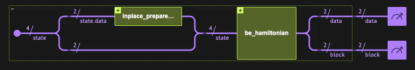
As a sanity check before the main algorithm, we verify the Hamiltonian block-encoding: we apply

U_H

on the initial state and check that the post-selected result matches

(H/\bar{\alpha})|\psi\rangle

as expected.

@qfunc
def main(data: Output[QNum[data_size]], block: Output[QNum[block_size]]):
    state = BlockEncodedState()
    allocate(state)

    inplace_prepare_amplitudes(state_to_evolve, 0.0, state.data)
    be_hamiltonian(state)
    bind(state, [data, block])


qprog_be = synthesize(main)
show(qprog_be)

Output:

Quantum program link: https://platform.classiq.io/circuit/3D345OwANKwFbd3NPhrzEpdKQHY
  

TOLERANCE = 1e-9
with ExecutionSession(qprog_be, execution_preferences=execution_preferences) as es:
    res_be = es.sample()

state_result_be = get_projected_state_vector(res_be)
expected_state_be = matrix @ state_to_evolve

renormalized_be, overlap_be = compare_quantum_classical_states(
    expected_state_be, state_result_be, BE_SCALING
)
print("Expected state:", expected_state_be)
print("Resulting state after rescaling:", renormalized_be)
assert np.isclose(overlap_be, 1, TOLERANCE)
print("=" * 40)
print(f"Fidelity is 1 (with {TOLERANCE} tolerance)")

Output:

Expected state: [0.48661409+0.j 0.20780411+0.j 0.06549975+0.j 0.04701937+0.j]
  Resulting state after rescaling: [0.48661409+4.76606469e-17j 0.20780411-4.89301046e-17j
   0.06549975-9.06290967e-17j 0.04701937+5.30017642e-17j]
  ========================================
  Fidelity is 1 (with 1e-09 tolerance)
  

Implementation

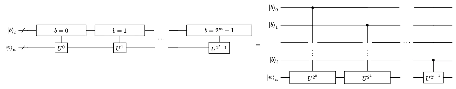
We build an LCU of the unitaries

\{W^k\}

with coefficients

\{\beta_k\}

. The select operator over a series of unitary powers is implemented efficiently: instead of applying

2^l

multi-controlled operations, we apply

l

single-controlled operations, where the

i

-th control qubit applies

W^{2^i}

(analogous to the QPE circuit structure).

@qfunc
def select_powered_unitaries(u: QCallable, block: QArray):
    repeat(block.len, lambda i: control(block[i], lambda: power(2**i, lambda: u())))

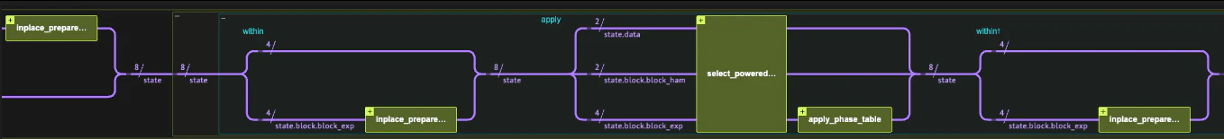
First, we define Quantum Structs for the Qubitization block-encoding. The block part, QubitizationBlock, contains the block variable from the Hamiltonian block-encoding, and a block variable on which we apply the PREPARE operation of the LCU to construct the sum of Chebyshev polynomials of

H

. The data variable follows that of the Hamiltonian encoding. In addition, we assemble the lcu_cheb function using prepare_select with the efficient select_powered_unitaries as the select operation.

class QubitizationBlock(QStruct):
    block_ham: QNum[block_size]
    block_exp: QNum[exp_block_size]


class QubitizationState(QStruct):
    data: QNum[data_size]
    block: QubitizationBlock


@qfunc
def lcu_cheb(
    coefs: list[float], be_qfunc: QCallable[BlockEncodedState], state: QubitizationState
):
    prepare_select(
        coefficients=coefs,
        select=lambda lcu_block: select_powered_unitaries(
            lambda: walk_operator(be_qfunc, [state.data, state.block.block_ham]),
            lcu_block,
        ),
        block=state.block.block_exp,
    )

The code in the rest of this section builds a model that applies the lcu_cheb function on the randomly prepared vector, synthesizes it, executes the resulting quantum program, and verifies the results.

@qfunc
def main(
    data: Output[QNum[data_size]], block: Output[QNum[block_size + exp_block_size]]
):
    state = QubitizationState()
    allocate(state)
    inplace_prepare_amplitudes(state_to_evolve, 0.0, state.data)

    lcu_cheb(exp_coeffs, be_hamiltonian, state)
    bind(state, [data, block])


qprog_cheb_lcu = synthesize(main, preferences=Preferences(optimization_level=1))
show(qprog_cheb_lcu)

Output:

Quantum program link: https://platform.classiq.io/circuit/3D34BcmBXo9yfTgz7rBvSylBdey
  

with ExecutionSession(qprog_cheb_lcu, execution_preferences) as es:
    results_cheb_lcu = es.sample()

state_result_cheb_lcu = get_projected_state_vector(results_cheb_lcu)
exp_scaling_factor_cheb_lcu = exp_be_scaling

renormalized_state_cheb_lcu, overlap_cheb_lcu = compare_quantum_classical_states(
    expected_state, state_result_cheb_lcu, exp_scaling_factor_cheb_lcu
)
print("Expected state:", expected_state)
print("Resulting state after rescaling:", renormalized_state_cheb_lcu)
assert np.linalg.norm(renormalized_state_cheb_lcu - expected_state) < EPS
print("=" * 40)
print("Overlap between expected and resulting state:", overlap_cheb_lcu)

Output:

Expected state: [-0.66939463-0.00189774j  0.58369085-0.33082778j  0.07045108-0.25195773j
   -0.12292945-0.13493516j]
  Resulting state after rescaling: [-0.66939463-0.00189774j  0.58369086-0.33082778j  0.07045109-0.25195773j
   -0.12292945-0.13493516j]
  ========================================
  Overlap between expected and resulting state: 1.0
  

References

[1]: Berry, D. W., Childs, A. M., & Kothari, R. Hamiltonian simulation with nearly optimal dependence on all parameters. In Proceedings of the 56th IEEE Symposium on Foundations of Computer Science (FOCS), pp. 792–809 (2015). [2]: Szegedy, M. Quantum speed-up of Markov chain based algorithms. In 45th Annual IEEE Symposium on Foundations of Computer Science, pp. 32–41 (2004). [3]: Lin, L. Lecture notes on quantum algorithms for scientific computation. arXiv:2201.08309 [quant-ph] (2022).

Technical Notes

Generalizing to Non-Hermitian Block-Encoding Unitaries

The current implementation assumes that the block-encoding unitary

U_H

is also Hermitian. This assumption underlies the walk operator’s spectral properties. For a non-Hermitian block-encoding unitary, an analogous walk operator can be defined as

\tilde{W} \equiv U_H^T \Pi_{|0\rangle_m} U_H \Pi_{|0\rangle_m}

, which satisfies equivalent spectral properties. See Section 7.4 in Ref. [3] for details.

Comparison with Other Methods

Method	extra block qubits	Controlled $U_H$ ?	Amplitude amplification?	Classical preprocessing
GQSP	1	Yes	No	Angle computation
QSVT	2	No	Yes (for a factor of 2)	Angle computation
Qubitization	$O(\log d)$	Yes	Yes (for the sum of Cheb. coefficients)	None

All three methods share the same asymptotic query complexity. Differences in the table reflect the detailed implementation of this specific example.

Algorithms

Applications

Functions

Tutorials

Hamiltonian Simulation with Qubitization (Chebyshev LCU)

View on GitHub

Preliminaries

Setting a Specific Hamiltonian to Evolve

Setting Up a Statevector Simulator

The Jacobi–Anger Expansion

The Walk Operator

Verifying the Block-Encoding

Implementation

References

Technical Notes

Generalizing to Non-Hermitian Block-Encoding Unitaries

Comparison with Other Methods

Algorithms

Applications

Functions

Tutorials

Documentation Index

View on GitHub

​Preliminaries

​

​Setting a Specific Hamiltonian to Evolve

​

​Setting Up a Statevector Simulator

​

​The Jacobi–Anger Expansion

​

​The Walk Operator

​

​Verifying the Block-Encoding

​Implementation

​References

​Technical Notes

​

​Generalizing to Non-Hermitian Block-Encoding Unitaries

​

​Comparison with Other Methods

Preliminaries

Setting a Specific Hamiltonian to Evolve

Setting Up a Statevector Simulator

The Jacobi–Anger Expansion

The Walk Operator

Verifying the Block-Encoding

Implementation

References

Technical Notes

Generalizing to Non-Hermitian Block-Encoding Unitaries

Comparison with Other Methods